Bootstrapping has always been an intriguing concept. The main idea is that resampling (with replacement) from a sample of data can give similar inference on a statistic as new draws from the population. The term refers to the ability of a single sample to make inference on a statistic with no other resources. This methodology always reminds me of the entrepreneurial phrase “pulling yourself up by your bootstraps”.
What is a Bootstrap?
A bootstrapped sample is a form of resampling from a single sample to approximate the true distributoin of a statistic. For example, suppose I want to know about the distribution of a sample mean, \(\bar{X}\). If it were possible to get a large number of samples from the population, each with their own \(\bar{X}\), it would be easy to look at the true distribution of \(\bar{X}\).
Samples from Population
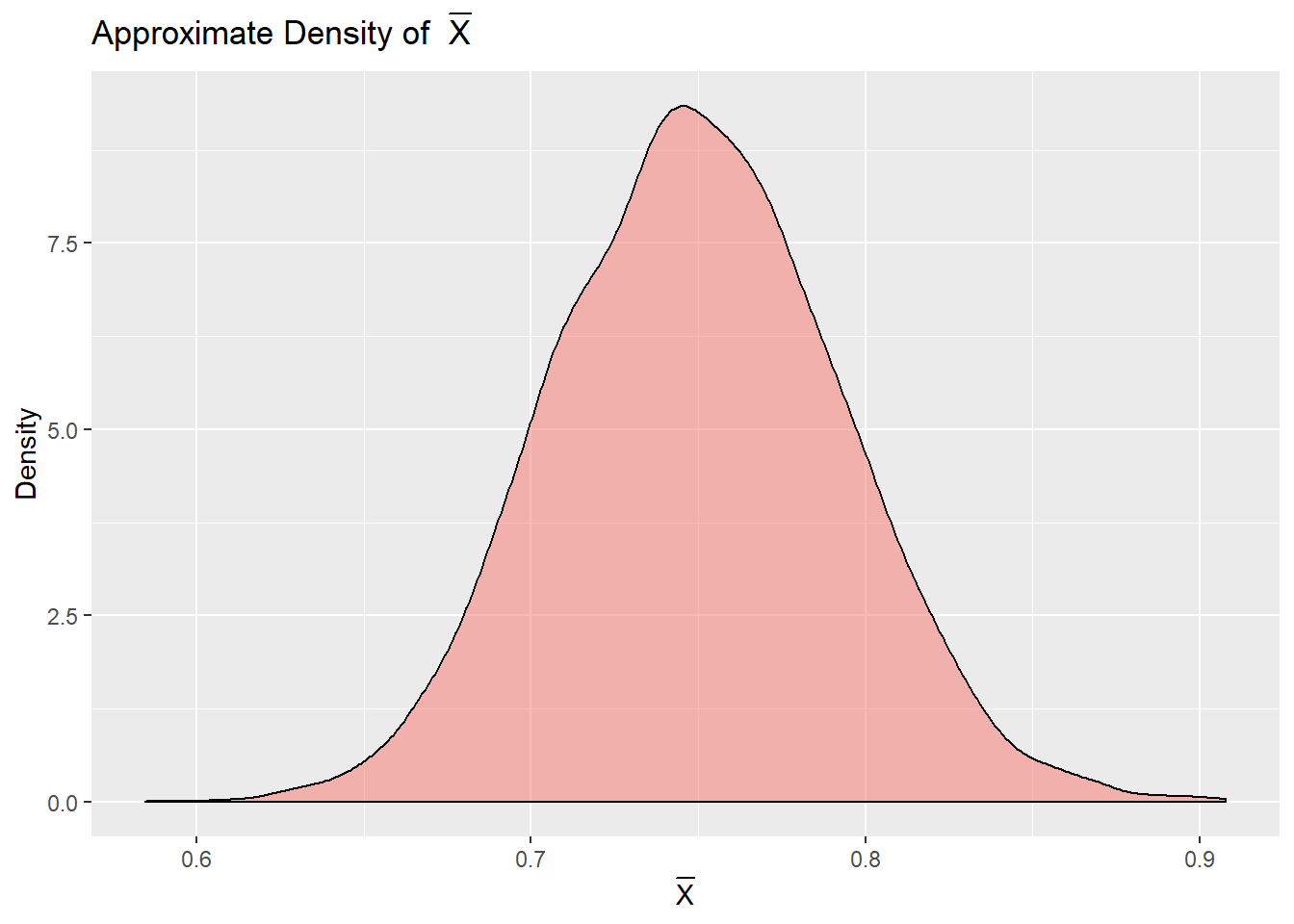
As an example, say we somehow come upon \(\bar{X}\) for \(10,000\) different samples of size \(100\) from a particular distribution. In this example, it will be from a \(Gamma(3,4)\). Below, the function, gamma.sample(), will get these samples. In practice, each sample is likely difficult to obtain, so this method is often not available.
gamma.sample <- function() rgamma(100,3,4)
xbars <- sapply(1:10000, function(x) mean(gamma.sample()))
The density of our \(\bar{X}\)s can give us a nice approximation to the true distribution of \(\bar{X}\). A density plot on these samples gives a good approximation to the truth.
Code for Above Density Plot
library(ggplot2)
library(reshape2)

xbars.df <- data.frame("Population" = xbars)
data <- melt(xbars.df)

ggplot(data,aes(x=value, fill=variable)) + geom_density(alpha=0.5) +
  xlab(expression(bar(X))) +
  ylab("Density") +
  ggtitle(expression(paste("Approximate Density of  ",bar(X)))) +
  theme(legend.position = "none")
Bootstrapped Samples
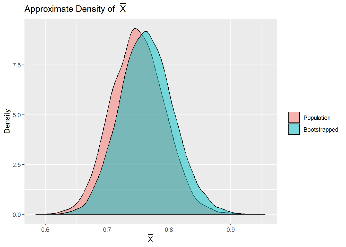
Actually getting \(10,000\) distinct samples from a population would be much more difficult than gathering a single sample. Amazingly, through the power of bootstrapping, it is possible to approximate the true distribution of \(\bar{X}\) with only a single sample! If we have \(10,000\) bootstrapped samples, they can also give a good approximation, without needing to resample from the population. Bootstrapped samples are sampled (with replacement) from a single sample. In the code, bootstrap.sample() is a function that samples with replacement from the sample, one.sample, giving a new, sample.
one.sample <- gamma.sample()
bootstrap.sample <- function() sample(one.sample, replace = TRUE)
boot.xbars <- sapply(1:10000, function(x) mean(bootstrap.sample()))
Using each bootstrapped sample as if it were a unique sample from the population is enough to approximate the true distribution of \(\bar{X}\).
Code for Above Density Plots
all.xbars <- data.frame("Population" = xbars, "Bootstrapped" = boot.xbars)
data <- melt(all.xbars)

ggplot(data,aes(x=value, fill=variable)) + geom_density(alpha=0.5) +
  xlab(expression(bar(X))) +
  ylab("Density") +
  ggtitle(expression(paste("Approximate Density of  ",bar(X)))) +
  theme(legend.title = element_blank())
When is Bootstrapping Helpful?
Bootstrapping may be useful for approximating the true distribution of \(\bar{X}\), but there are practical examples to when bootrapping can be useful. This method can help with confidence intervals, prediction intervals, hypothesis tests, or other measurements of uncertainty for statistics when it may be difficult or impossible to obtain in closed form.
Example: Prediction in Simple Linear Regression
To start, say we have samples from a simple linear model, \(y_i=\beta_0 + x_i\beta_1+\epsilon_i\), where \(\epsilon_i\sim N(0,\sigma^2)\). Fortunately, we know that a prediction, \(\hat{y}\), on a new \(x^\star\) is normally distributed. In fact, \(\hat{y}\sim N(\beta_0+x^\star\beta_1,\sigma^2)\). Because we know this distribution, we can estimate \(\hat{\beta_0}\), \(\hat{\beta_1}\), and \(\hat{\sigma}^2\) to give approximate prediction intervals on \(\hat{y}\).
In the code below, we have \(100\) samples from the true model \(y_i=5+x_i*2+\epsilon_i\), where \(\epsilon_i\sim N(0,.75^2)\).
beta0 <- 5
beta1 <- 2
n <- 100
sigma <- .75

x <- runif(n)
epsilon <- rnorm(n, 0, sd = sigma)
y <- beta0 + x * beta1 + epsilon
If we fit a standard linear model, with assumptions of normality, we can see that the estimates for \(\hat{\beta_0}\), \(\hat{\beta_1}\), and \(\hat{\sigma}^2\) are pretty close to the true values, giving decent approximations for predictions and prediction intervals.
lin.model <- lm(y~x)

betahat <- as.numeric(lin.model$coefficients)
sigmahat <- summary(lin.model)$sigma

betahat
## [1] 4.949982 2.151056sigmahat## [1] 0.7212661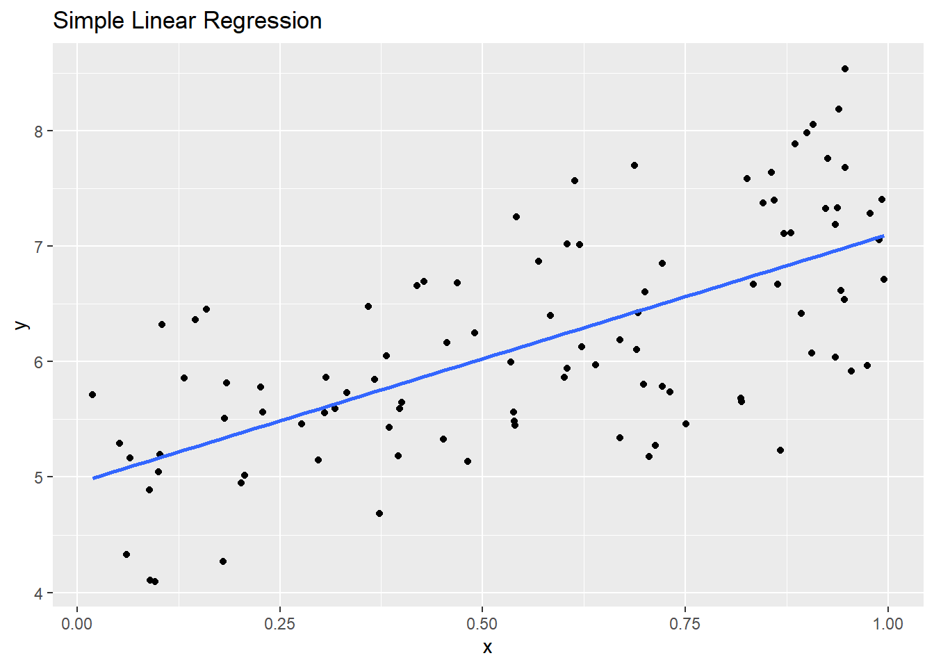
Code for Above Plot
library(ggplot2)
data <- data.frame(y,x)
ggplot(data, aes(y=y, x=x)) +
  geom_point() +
  geom_smooth(method = 'lm', se = FALSE) +
  ggtitle("Simple Linear Regression")
From these estimates, we can get the approximated distribution of a new \(y\), given any \(x\) value. In this example, we have \(x=.85\). Theory tells us that \(y|x\dot{\sim} N(\hat{\beta_0} + x\hat{\beta_1},\hat{\sigma}^2)\). From this, we can get a \(95\%\) prediction interval for \(y\), given the new \(x\).
xnew <- .85
ypred <- betahat[1] + xnew * betahat[2]

pred.int <- ypred + qnorm(c(.025, .975), 0, sd = sigmahat)
ypred
## [1] 6.778379pred.int## [1] 5.364724 8.192035If we knew the true distribution of \(y_i\), the prediction interval for the new \(y\) would be exact.
ypred.true <- beta0 + xnew * beta1

true.pred.int <- qnorm(c(.025,.975), ypred.true, sd = sigma)
ypred.true
## [1] 6.7true.pred.int## [1] 5.230027 8.169973Suppose that we knew nothing about the true distribution of \(\epsilon_i\), obtaining a prediction interval for the new \(y\) would be impossible. Let us ignore this assumption for this case and use bootstrapping instead. First, we would need to get bootstrapped samples of the residuals from a linear model.
boot.resid.sample <- function() {
  boot.index <- sample(1:n, replace = TRUE)
  boot.resid <- residuals(lin.model)[boot.index]
  return(boot.resid)
}

boot.resids <- lapply(1:1000, function(x) boot.resid.sample())
These bootstrapped residuals can be used to approximations for both the expected \(\hat{y}\), and its prediction interval. By bootstrapping, we have avoided the normality assumption entirely and gotten very similar prediction intervals to those when assuming normality.
this.pred <- c()
pred.lwr.pi <- c()
pred.upr.pi <- c()

for(i in 1:1000){
  pred.lwr.pi[i] <- ypred + as.numeric(quantile(boot.resids[[i]], .025))
  pred.upr.pi[i] <- ypred + as.numeric(quantile(boot.resids[[i]], .975))
}

boot.pred.int <- c(mean(pred.lwr.pi), mean(pred.upr.pi))

ypred
## [1] 6.778379boot.pred.int## [1] 5.601059 8.014272For normally distributed residuals, bootstrapping a prediction interval isn’t particularly helpful. What if the residuals are not normally distributed? The assumptions earlier that provided the approximate distribution (and therefore prediction intervals) of \(\hat{y}\) no longer apply. Without bootstrapping, we would be at a loss for how to get prediction intervals on a new \(y\), especially if the distribution of the residuals was unknown entirely.
Let us generate samples through the same example as above, but with \(\epsilon_i\sim Unif(-1,1)\).
epsilon <- runif(n, -1, 1)
y <- beta0 + x * beta1 + epsilon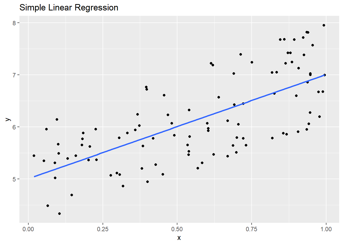
Code for Above Plot
library(ggplot2)
data <- data.frame(y,x)
ggplot(data, aes(y=y, x=x)) +
  geom_point() +
  geom_smooth(method = 'lm', se = FALSE) +
  ggtitle("Simple Linear Regression")
The mean predictions form a linear model (assuming normality) are still valid, but now the prediction interval must be bootstrapped.
lin.model <- lm(y~x)
betahat <- as.numeric(lin.model$coefficients)
ypred <- betahat[1] + xnew * betahat[2]

boot.resids <- lapply(1:1000, function(x) boot.resid.sample())

this.pred <- c()
pred.lwr.pi <- c()
pred.upr.pi <- c()

for(i in 1:1000){
  pred.lwr.pi[i] <- ypred + as.numeric(quantile(boot.resids[[i]], .025))
  pred.upr.pi[i] <- ypred + as.numeric(quantile(boot.resids[[i]], .975))
}

boot.pred.int <- c(mean(pred.lwr.pi), mean(pred.upr.pi))

ypred
## [1] 6.706305boot.pred.int## [1] 5.800791 7.668947Because we manufactured this data, we can still get the true prediction intervals and compare to the bootstrapped intervals. The bootstrapped prediction intervals are reasonable approximations for the true prediction intervals.
ypred.true## [1] 6.7ypred.true + qunif(c(.025,.975), -1, 1)## [1] 5.75 7.65The times that bootstrapping come in handy for me is when I am using a model that has no distributional asusmptions. For example, when I use Lasso regression, there is no closed-form solution to confidence intervals on \(\hat{\boldsymbol{\beta}}\) or to prediction intervals. These are both intervals that can be bootstrapped with no distributional assumptions. Bootstrapping can also help in ridge regression, time series analysis (and other correlated data), or whenever one is not confident about the underlying distributional characteristics of a model. Even when theory is available for “better” estimates, bootstrapping can still be a reasonable approximation.
Anytime the distribution of a sample statistic is not known, bootstrapping can be used to approximate the distribution of the sample statistic. If one is interested in the true distribution of the median, minimum, or any other sample statistic, bootstrapping can be the way to go.